Tutorial 8: Geometry Mapping and Tessellation
- Part 1: Normal Mapping
- Part 2: Parallax Occlusion Mapping
- Part 3: PN Triangle Tessellation
- Extra:
- Super Extra:
This tutorial covers how to add normal and parallax mapping. It also covers creating tessellation shaders and using them with PN Triangle tessellation.
This tutorial will continue on from the last by extending the previously created code. It is assumed that you have created a copy of last tutorial’s code that can be used for the remainder of this one.
Part 1: Normal Mapping
Lighting equations all determine reflected/transmitted light based on the normal to the surface. Since only the normal is being used the actual underlying geometry has little to do with determining the surfaces appearance. By varying the surface normal across a single face the surface can be given the appearance of having more topology than it actually does. Normal Mapping is a technique used to vary the normal across a surface without affecting its geometry. A Normal Map is used to store the actual surface normal within a texture. During rendering instead of using the geometric normal the surfaces UV coordinates are used to fetch the stored normal from the texture. This returned normal is then used for all lighting calculations.
Since the surface of an object moves around within the scene the values in the normal map cannot be world space directions. Instead tangent space is used to define the normal. Tangent space is simply a coordinate space that is relative to the surface of the geometry. This way no matter how the geometry is actually oriented in the world the surface space will always be the same. Using tangent space normals requires converting them to world space.
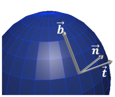
Tangent space is an orthogonal coordinate system defined by a surfaces tangent vector \(\overrightarrow{\mathbf{t}}\), bitangent (sometimes referred as binormal) vector \(\overrightarrow{\mathbf{b}}\) and normal \(\overrightarrow{\mathbf{n}}\).
A tangent to world space transform \(M_{T \rightarrow W}\) can be determined from the world space tangent vector \(\overrightarrow{\mathbf{t}}\), bitangent vector \(\overrightarrow{\mathbf{b}}\) and normal \(\overrightarrow{\mathbf{n}}\):
\[M_{T \rightarrow W} = (\begin{matrix} (\overrightarrow{\mathbf{t}}) & (\overrightarrow{\mathbf{b}}) & (\overrightarrow{\mathbf{n}}) \\ \end{matrix})\]The final normal \({\overrightarrow{\mathbf{n}}}^{'}\) is calculated by converting the normal mapped normal \({\overrightarrow{\mathbf{n}}}_{T}\) to a normalized signed vector and then transforming from tangent space.
\[{\overrightarrow{\mathbf{n}}}^{'} = M_{T \rightarrow O}*(\left( {\overrightarrow{\mathbf{n}}}_{T} - 0.5 \right)*2)\]- Normal mapping requires having a tangent and bitangent direction vector. The bitangent can be calculated as the cross product of the normal and the tangent so we only need the tangent vector for the surface. Much like the surface normal this needs to be passed into the vertex shader. To do this we need to add tangent inputs and outputs to our existing vertex and geometry shaders (Note: the shaders used for shadow mapping don’t need tangents as they do not perform lighting). Vertex shaders need to be updated to pass through the transformed tangent vector. Since we already have 3 inputs we need to use the next available location.
...
layout(location = 3) in vec3 v3VertexTangent;
...
layout(location = 3) smooth out vec3 v3TangentOut;

void main() {
    ...
    // Transform tangent
    vec4 v4Tangent = m4Transform * vec4(v3VertexTangent, 0.0f);
    v3TangentOut = v4Tangent.xyz;
    ...
- Update the geometry shader used for reflection mapping so that it has the new tangent inputs and outputs. Just like for the normal each invocation needs to transform the tangent based on the view-projection transform.
- To use the passed in tangent we now need to add a new input to the Fragment shader. We also need to add a new texture sampler that will hold the normal map texture using the next available binding (here it is 9).
layout(location = 3) in vec3 v3TangentIn;
...
layout(binding = 9) uniform sampler2D s2NormalTexture;
- To use normal mapping, we need to add a new function to our Fragment shader that will read the normal in from a texture file and then convert it to world space. This function will take the tangent, normal, bitangent and current UV coordinates as input. It will then use the current UV values to read in the value from texture. The normal map supplied with this tutorial uses BC5 texture compression as it provides the best quality for normal maps out of the current hardware compression schemes. This compresses a normal using only 2 components (the ‘x’ and ‘y’) so the 3rd component needs to be recalculated. Since the normal is stored with unit length we can calculate the 3rd component such that the vector length will be ‘1’. Once the normal is calculated we then transform it from tangent space to world space.
vec3 normalMap(in vec3 v3Normal, in vec3 v3Tangent, in vec3 v3BiTangent, in vec2 v2LocalUV)
{
    // Get normal map value
    vec2 v2NormalMap = (texture(s2NormalTexture, v2LocalUV).rg - 0.5f) * 2.0f;
    vec3 v3NormalMap = vec3(v2NormalMap, sqrt(1.0f - dot(v2NormalMap, v2NormalMap)));

    // Convert from tangent space
    vec3 v3RetNormal = mat3(v3Tangent, v3BiTangent, v3Normal) * v3NormalMap;
    return normalize(v3RetNormal);
}
- In the main function of the Fragment shader we now need to call the new normal map function. To do this we must first calculate the bitangent direction which is just the cross product of the normal and the tangent (where
v3Tangentis the input tangent normalized). We replace the existing normal with the result of the normal map function which will then get used for all future lighting calculations.
// Generate bitangent
vec3 v3BiTangent = cross(v3Normal, v3Tangent);

// Perform Bump Mapping
v3Normal = normalMap(v3Normal, v3Tangent, v3BiTangent, v2UVIn);
- Now we need to pass the new tangent data into the shaders in order to use them. This requires updating the existing vertex description to also include per-vertex tangent information. This will be stored much like the vertex normal.
struct CustomVertex
    ...
    vec3 v3Tangent;
};
- Now within the scene loading function we need to update the way meshes are loaded and stored. We have already told Assimp to ensure that meshes are loaded with tangent information so all we have to do is to read this data from Assimp and store it in our vertex buffer. Once loaded we then need to tell OpenGL that there is now an additional attribute in the vertex array.
p_vBuffer->v3Tangent = vec3(p_AIMesh->mTangents[j].x,
                            p_AIMesh->mTangents[j].y,
                            p_AIMesh->mTangents[j].z);
...
glVertexAttribPointer(3, 3, GL_FLOAT, GL_FALSE, sizeof(CustomVertex), (const GLvoid *)offsetof(CustomVertex, v3Tangent));
glEnableVertexAttribArray(3);
- Next we need to add code to the material loading section to load the correct normal map. To do this we need to add a new variable to the material type. This texture can be loaded by getting the texture from Assimp in the exact same way we have been doing previously. The only difference is that this time the texture type is specified as
aiTextureType_NORMALS(remember to generate an extra texture).
struct MaterialData
{
    ...
    GLuint m_uiNormal;
    ...
};
- Make sure to add an identical variable to the object type
ObjectDataand then set it during the load scene node functionGL_LoadSceneNodeidentically to how we have done previously.
- Finally, we just need to add code within the render object function to make sure that the texture is bound to the corresponding texture location. This should be added directly after the existing per-object texture bindings.
glActiveTexture(GL_TEXTURE9);
glBindTexture(GL_TEXTURE_2D, p_Object->m_uiNormal);
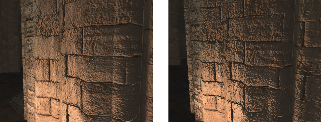
- You should now be able to run the program and compare the difference that adding normal maps make.
Part 2: Parallax Occlusion Mapping
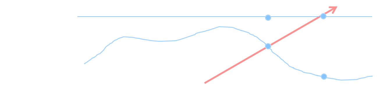
Normal mapping techniques fail to compensate for parallax effects which result from the angle the surface is viewed at. This is a result of retrieving the modified normal based on the geometric position being viewed \(\mathbf{p}_{a}\) which differs from the actual position when the view direction is not perpendicular to the surface. Since a normal map represents surface variation the equivalent surface position would actually be \(\mathbf{p}_{b}\). To determine the actual surface position a parallax map (a type of heightmap defining the height below the surface) is added which can be used to determine the surface topology.
Parallax Occlusion mapping works by breaking the total height range into a discrete number of steps. Starting at the initial point \(\mathbf{p}_{a}\) a parallax map is checked and if the resulting new point \(\mathbf{p}_{a}^{'}\) is greater than the current point then the UV coordinates are modified by moving down to the next step.
At each step the new texture coordinates \({(u,v)}_{i}^{'}\) for step \(i\) are determined from the number of steps \(n_{s}\) and the tangent space view vectors x/y components \({\overrightarrow{\mathbf{v}}}_{\{ x,y\}}^{T}\) and z component \({\overrightarrow{\mathbf{v}}}_{\{ z\}}^{T}\) such that:
\[{(u,v)}_{i}^{'} = {(u,v)}_{i - 1}^{'} + \frac{ {\overrightarrow{\mathbf{v}}}_{\{ x,y\}}^{T}}{- {\overrightarrow{\mathbf{v}}}_{\{ z\}}^{T}*n_{s}}\]where \({(u,v)}_{0}^{'} = 0\)
Once a new parallax map point is found that is higher than the current step height then recursion stops. If recursion stopped at step \(i\) then the final UV coordinates are determined by interpolating between the step height at \(i\) and \(i - 1\).
\[{(u,v)}_{}^{'} = {(u,v)}_{i - 1}^{'}w_{i} + (u,v)_{i}^{'}(1 - w_{i})\]where the weight \(w_{i}\) is calculated from the parallax map height \(f_{h}((u,v)_{i}))\) and the step height \(h_{i}\):
\[w_{i} = \frac{f_{h}((u,v)_{i})) - h_{i}}{(f_{h}((u,v)_{i})) - h_{i}) - f_{h}((u,v)_{i - 1})) - h_{i - 1}}\]This gives a new UV coordinate value which corresponds to the point on the surface that the view direction actually intersects with based on the surfaces parallax map. The new UV value is then used for all future texture lookups.
- To use Parallax Occlusion mapping we need to add an additional texture input to the Fragment shader that contains the parallax map data. We also need to scale the heightmap to fit the current surface. For this we need to add an additional input uniform that will hold the scale value.
layout(binding = 10) uniform sampler2D s2BumpTexture;

layout(location = 3) uniform float fBumpScale;
- To use Parallax Occlusion mapping we will add a new function to our Fragment shader. This function will take as inputs the 3 basis vectors used to define tangent space as well as the view direction. The first step is then to determine the tangent space view direction vector. We can then use the length of this vector to determine the number of steps we should take. If the tangent space view vector is parallel to the surface normal, then there will be no parallax effects to worry about. However, the further away from the normal the view direction is then the more steps we should add. Once the number of layers is determined we can then calculate the change in height and UV coordinates for each layer.
vec2 parallaxMap(in vec3 v3Normal, in vec3 v3Tangent, in vec3 v3BiTangent, in vec3 v3ViewDirection)
{
    // Get tangent space view direction
    vec3 v3TangentView = vec3(dot(v3ViewDirection, v3Tangent),
         dot(v3ViewDirection, v3BiTangent), dot(v3ViewDirection, v3Normal));
    v3TangentView = normalize(v3TangentView);

    // Get number of layers based on view direction
    const float fMinLayers = 5.0f;
    const float fMaxLayers = 15.0f;
    float fNumLayers = round(mix(fMaxLayers, fMinLayers, abs(v3TangentView.z)));

    // Determine layer height
    float fLayerHeight = 1.0f / fNumLayers;
    // Determine texture offset per layer
    vec2 v2DTex = fBumpScale * v3TangentView.xy / (v3TangentView.z * fNumLayers);

    // *** Add remaining Parallax Occlusion code here ***
}
- Next, we get the current height from the heightmap texture. In this tutorial we will use standard bump maps as the input heightmap where the larger the value in the heightmap the higher the corresponding point. Unlike standard heightmaps however we will limit the maximum heightmap value so that it corresponds to the height of the surface. This way any heightmap values less than the maximum will be below the surface and no value can be above the surface. Since we are not actually modifying the geometry any height above the surface can’t actually be visualised so to improve performance and quality, we deliberately prevent such values. We then loop through each step and check the height in the texture against the height of the view vector at each step. If we find a location where the heightmap is higher than the position on the view direction, then we stop looping. In order to support dynamic branching, we use a special form of texture fetch called
textureGrad. This allows retrieving from a mipmap level based on a specified coverage. Normally this is done automatically by OpenGL by taking the distance between the current fragment and a neighbouring fragments texture fetch operation. However, within the loop we want each fragment to be able to exit at any point without requiring neighbouring fragments to be in the same position in code. So, we manually specify the gradients so that OpenGL doesn’t require there to be a neighbouring pixel executing the same code.
// Get texture gradients to allow for dynamic branching
vec2 v2Dx = dFdx(v2UVIn);
vec2 v2Dy = dFdy(v2UVIn);

// Initialise height from texture
vec2 v2CurrUV = v2UVIn;
float fCurrHeight = textureGrad(s2BumpTexture, v2CurrUV, v2Dx, v2Dy).r;

// Loop over each step until lower height is found
float fViewHeight = 1.0f;
float fLastHeight = 1.0f;
vec2 v2LastUV;
for (int i = 0; i < int(fNumLayers); i++) {
    if(fCurrHeight >= fViewHeight)
        break;
    // Set current values as previous
    fLastHeight = fCurrHeight;
    v2LastUV = v2CurrUV;
    // Go to next layer
    fViewHeight -= fLayerHeight;
    // Shift UV coordinates
    v2CurrUV -= v2DTex;
    // Get new texture height
    fCurrHeight = textureGrad(s2BumpTexture, v2CurrUV, v2Dx, v2Dy).r;
}
- Finally, once we have found the step where the view direction is blocked by the surface height, we then need to interpolate between this and the last value to get a closer approximation to the actual intersection point. At each point in the loop we stored the height from the previous step so all we need to do is to interpolate between the 2 heights based on the distance between each height and the view direction vector.
// Get heights for linear interpolation
float fNextHeight = fCurrHeight - fViewHeight;
float fPrevHeight = fLastHeight - (fViewHeight + fLayerHeight);

// Interpolate based on height difference
float fWeight = fNextHeight / (fNextHeight - fPrevHeight);
return mix(v2CurrUV, v2LastUV, fWeight);
- Now that the Parallax Occlusion function is complete we just need to add the code into the Fragment shaders main function that will call the new function. This will return a new UV coordinate value that should be used for all future texture lookups. Modify the normal map function call so that the new UV value is passed in instead. Also update all the existing texture lookups for diffuse, specular etc. textures to use the new UV values.
// Perform Parallax Occlusion Mapping
vec2 v2UVPO = parallaxMap(v3Normal, v3Tangent, v3BiTangent, v3ViewDirection);
- In the host code we now need to load in the heightmap texture. Just like with the previous normal map value we need to add new variables to
MaterialDataand corresponding variables toObjectData. We can then add code to the scene loading function to load the new texture. As we are using a heightmap this texture can be retrieved from Assimp usingaiTextureType_DISPLACEMENTto get the parallax map. Similar to how we have previously retrieved transparency and reflectivity values from Assimp we can then retrieve the bump scaling factor usingAI_MATKEY_BUMPSCALING. Also, remember to add code toGL_LoadSceneNodeto ensure that each object has a copy of the bump map texture and scale. Finally add code to the render object’s function that binds the new texture to the corresponding texture binding (in this case it is 10) and updates the scaling uniform (in this case it’s at location 3).
struct MaterialData
{
    ...
    GLuint m_uiBump;
    ...
    float m_fBumpScale;
};
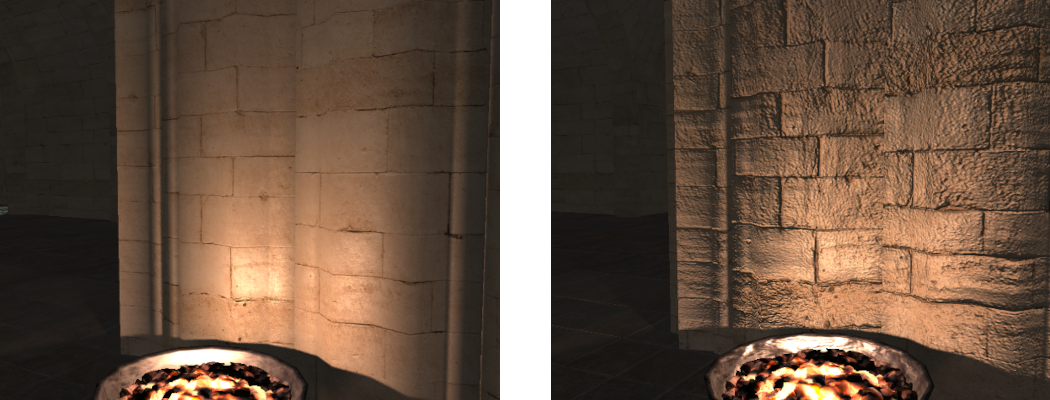
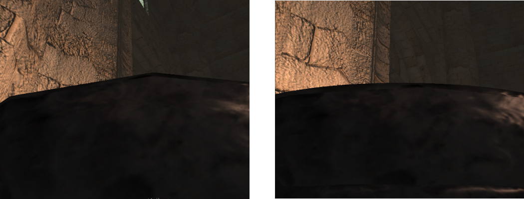
- You should now be able to compile and run your code to see the effect of Parallax Occlusion mapping.
Part 3: PN Triangle Tessellation
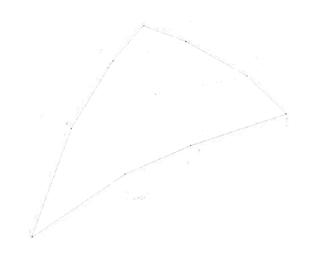
Point-Normal (PN) Triangles is a technique used to add additional surface geometry by smoothing out a surface. Each triangle in the mesh is replaced by a special form of a Bezier patch called a Bezier Triangle. The surface is then tessellated by filling in points across the triangle based on the curved surface of the new Bezier Triangle. This gives each triangle a slightly puffy surface based on the deviation of the normals at each of the triangles vertices.
A Bezier Triangle is defined in barycentric coordinates \(\alpha\), \(\beta\), \(\gamma\) as:
\[C(\alpha,\ \beta,\ \gamma) = \ \sum_{i + j + k = 3}^{}{\mathbf{p}_{i,\ j,k}\frac{3!}{i!j!k!}\alpha^{i}\beta^{j}\gamma^{k}}\]\(C(\alpha,\ \beta,\ \gamma) = \mathbf{p}_{300}\gamma^{3} + \mathbf{p}_{030}\alpha^{3} + \mathbf{p}_{003}\beta^{3} +\) \(\mathbf{p}_{210}3\gamma^{2}\alpha + \mathbf{p}_{120}3\gamma^{2}\alpha + \mathbf{p}_{201}3\gamma^{2}\beta +\) \(\mathbf{p}_{021}3\alpha^{2}\beta + \mathbf{p}_{102}3\gamma\beta^{2}\alpha + \mathbf{p}_{012}3\alpha^{2}\beta + \mathbf{p}_{111}6\gamma\alpha\beta\)
To generate each of the new points \(\mathbf{p}_{i,\ j,k}\) requires several steps. The original vertices of the triangle remain unchanged and are named \(\mathbf{p}_{300},\mathbf{p}_{030},\mathbf{p}_{003}\). Two midpoints are generated on each edge; one 1/3 of the way and the other 2/3 of the way along the edge. Each midpoint is projected onto the plane created by the nearest vertex and its associated vertex normal. The position of \(\mathbf{p}_{111}\) is calculated from the vector from the original triangle centre (average of the three original vertices) to the average of the 6 new midpoints. The new position is found half way along this new vector.
Tessellation can be performed within OpenGL using the inbuilt Tessellation shader stages. Tessellation in OpenGL has 3 stages; Tessellation Control Stage, Tessellator Stage and Tessellation Evaluation Stage.
The Tessellation Control Stage is a programmable shader stage that takes the input control points/vertices and determines how the input patch should be tessellated along each of the patches edges. This stage can be used for Continuous Level of Detail (CLOD) algorithms to determine how best to tessellate each edge of the input patch in order to achieve the best compromise between detail and performance. The output from this stage should be values used to describe how many new tessellated points should be generated for the input patch.
The Tessellator Stage is a fixed function pipeline stage that takes the inputs from the Control stage and creates a sampling pattern of the domain that represents the geometry patch and generates a set of smaller objects (triangles, points, or lines) that connect these samples. For instance, when tessellating triangles this stage will take as input the number of tessellations along each of the 3 edges and will output the actual barycentric coordinates for each of the new tessellated coordinates.
The Tessellation Evaluation Stage is a programmable shader stage that takes the inputs from the Tessellator stage and calculates the corresponding vertex positions. The Evaluation shader is run once for each generated output sample and is responsible for generating a single output vertex based on its input tessellation values.
- To use tessellation in OpenGL we need to create 2 new shaders. The first of which is the Control shader. This shader will take the outputs of the vertex shader based on the number of control points in a patch. In this case a patch is just a triangle so the number of inputs is 3. We will use the
layout(vertices) outqualifier to specify that this shader should be run 3 times. Since we have 3 input vertices we will run the shader once for each of them. The shader then takes as input an array of vertices (which in this case will hold 3 values) for each of the outputs from the vertex shader. The shader will then pass through each of these values in output arrays. Since we are only processing triangles there are only 3 values in each output array so we specify the array size (note: This should not be done on inputs). Lastly the shader needs to determine the PN Triangle control points that will be used to tessellate the surface in the later shader stage. Note that the layout locations increase by 3 for each new array. This is because each output array contains 3 elements and so it occupies 3 output locations. The last output is a single control point. This point will only be calculated by 1 of the shader invocations so we specify that only 1 shader will work on it withpatch.
#version 430 core

layout(vertices = 3) out;

// Inputs from vertex shader
layout(location = 0) in vec3 v3VertexPos[];
layout(location = 1) in vec3 v3VertexNormal[];
layout(location = 2) in vec2 v2VertexUV[];
layout(location = 3) in vec3 v3VertexTangent[];

// Passed through outputs
layout(location = 0)  out vec3 v3PositionOut[3]; //030, 003, 300
layout(location = 3)  out vec3 v3NormalOut[3];
layout(location = 6)  out vec2 v2UVOut[3];
layout(location = 9)  out vec3 v3TangentOut[3];
// PN Triangle additional data
layout(location = 12) out vec3 v3PatchE1[3];  //021, 102, 210
layout(location = 15) out vec3 v3PatchE2[3];  //012, 201, 120
layout(location = 18) out patch vec3 v3P111;

void main()
{
    // *** Add Control shader code here ***
}
- Within the shaders main function, we first need to pass-through the existing input vertex attributes as these will be used as part of the PN Triangle code later. Since we specified that the shader should be run 3 times in parallel then each invocation of the shader only needs to pass-through 1 of the input values (as the other 2 invocations will pass through the others). We use
gl_InvocationIDto determine which is the current invocation and then pass-through the corresponding input.
// Pass through the control points of the patch
v3PositionOut[gl_InvocationID] = v3VertexPos[gl_InvocationID];
v3NormalOut[gl_InvocationID] = v3VertexNormal[gl_InvocationID];
v2UVOut[gl_InvocationID] = v2VertexUV[gl_InvocationID];
v3TangentOut[gl_InvocationID] = v3VertexTangent[gl_InvocationID];
- Next we need to calculate the output PN Triangle control points. These points are passed out in 2 arrays each of 3 element lengths. Since the shader is invoked 3 times then each invocation only needs to calculate one element of each of these arrays. This requires determining the points 1/3 the way along the edge from the current point to the next point and vice versa. If each shader invocation calculates the 2 points between the current invocation point and the next, then between all 3 invocations all 6 required points will be generated.
// Calculate Bezier patch control points
const int iNextInvocID = gl_InvocationID < 2 ? gl_InvocationID + 1 : 0;
vec3 v3CurrPos = v3VertexPos[gl_InvocationID];
vec3 v3NextPos = v3VertexPos[iNextInvocID];
vec3 v3CurrNormal = normalize(v3VertexNormal[gl_InvocationID]);
vec3 v3NextNormal = normalize(v3VertexNormal[iNextInvocID]);

// Project onto vertex normal plane
vec3 v3ProjPoint1 = projectToPlane(v3NextPos, v3CurrPos, v3CurrNormal);
vec3 v3ProjPoint2 = projectToPlane(v3CurrPos, v3NextPos, v3NextNormal);

// Calculate Bezier CP at 1/3 length
v3PatchE1[gl_InvocationID] = ((2.0f * v3CurrPos) + v3ProjPoint1) / 3.0f;
v3PatchE2[gl_InvocationID] = ((2.0f * v3NextPos) + v3ProjPoint2) / 3.0f;
- Generating each of the new control points requires a new function that calculates the projection of each point onto the plane defined by the input vertices position and normal.
vec3 projectToPlane(in vec3 v3Point, in vec3 v3PlanePoint, in vec3 v3PlaneNormal)
{
    // Project point to plane
    float fD = dot(v3Point - v3PlanePoint, v3PlaneNormal);
    vec3 v3D = fD * v3PlaneNormal;
    return v3Point - v3D;
}
- The shader now needs to calculate the final centre control point. There is only one of these so only one of the shader invocations needs to actually calculate it. So we only allow the first invocation to perform the calculations. Since the calculation of the centre control point requires knowledge of the other control points we must wait for all other shader invocations to finish calculating their output values before we can continue. We do this by adding a barrier before continuing. After the barrier we then retrieve all the points calculated by all the invocations. We then average the 3 original points and then average the 6 new midpoints. We create the centre point based on the half length of the vector between these 2 averages.
barrier();
if (gl_InvocationID == 0) {
    // Get Bezier patch values
    vec3 v3P030 = v3VertexPos[0];
    vec3 v3P021 = v3PatchE1[0];
    vec3 v3P012 = v3PatchE2[0];
    vec3 v3P003 = v3VertexPos[1];
    vec3 v3P102 = v3PatchE1[1];
    vec3 v3P201 = v3PatchE2[1];
    vec3 v3P300 = v3VertexPos[2];
    vec3 v3P210 = v3PatchE1[2];
    vec3 v3P120 = v3PatchE2[2];

    // Calculate centre point
    vec3 v3E = (v3P021 + v3P012 + v3P102 + v3P201 + v3P210 + v3P120) / 6.0f;
    vec3 v3V = (v3P300 + v3P003 + v3P030) / 3.0f;
    v3P111 = v3E + ((v3E - v3V) / 2.0f);

    // *** Add tessellation level outputs here ***
}
Dynamic Tessellation can be used with a LOD scheme to tessellate a surface based on its current screen space coverage. Continuous LOD is a scheme that allows for a surface to have varying LOD levels across it. This is required for surfaces that stretch from close to far away from the camera. CLOD requires each edge in the tessellated surface to align which requires adaptively specifying a LOD for each triangle. CLOD can be achieved by measuring the clip space length of each edge. Based on the coverage each edge can be given a different tessellation factor. Since edges are shared between neighbouring triangles tessellation will be continuous across the whole surface.
When determining edge tessellation factors an edges clip space depth length should also be taken into account. Otherwise an edge nearly parallel to the view direction will have zero screen coverage and not be tessellated. This means any height displacement due to tessellation will not be observed. A solution is to ensure the calculated screen coverage is based on the length of the edge.
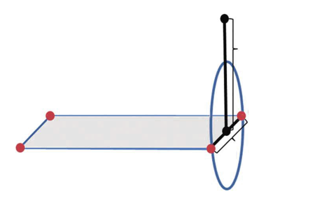
This can be achieved by projecting the size of a sphere with diameter equal to the length of the edge of the patch. To compute the projected size of the sphere the edge’s length is calculated. Then, compute 2 new points; the midpoint of the edge and a new point above this midpoint displaced by the edge’s length. The distance between the 2 points in clip space provides diameter of the enclosing sphere.
- The last step is to calculate the output tessellation values that will be used by the Tessellator stage. Since we are working on triangle patches we need to output 3 outer tessellation values corresponding to each of the 3 edges. Where the first output outer tessellation level is for the first edge and so forth. We then need to output a single inner tessellation level which corresponds to the number of inner rings to create within the triangle patch. We will use a projected sphere CLOD scheme to determine the tessellation level for each edge. The inner level is then the maximum of each of the outer levels. To calculate the LOD we need to know the edges screen coverage. This is found in the input position that was output from the vertex shader in view-projection space. This value is found in the implicit default input array
gl_inundergl_Position.
// Calculate the tessellation levels
gl_TessLevelOuter[0] = tessLevel(gl_in[1].gl_Position.xyz, gl_in[2].gl_Position.xyz);
gl_TessLevelOuter[1] = tessLevel(gl_in[2].gl_Position.xyz, gl_in[0].gl_Position.xyz);
gl_TessLevelOuter[2] = tessLevel(gl_in[0].gl_Position.xyz, gl_in[1].gl_Position.xyz);
gl_TessLevelInner[0] = max(gl_TessLevelOuter[0], max(gl_TessLevelOuter[1], gl_TessLevelOuter[2]));
- For the above code to work we need to add a new function to calculate the tessellation levels based on the projected sphere CLOD algorithm. This algorithm needs to know the ideal number of pixels that each output triangle should cover. This value should not be too small as otherwise output triangles will be smaller than a pixel and not visible. A value to large will defeat the purpose of using tessellation in the first place. A good value is around 4. The algorithm will then use an input uniform which contains the actual screen resolution. Based on this input resolution it will try and determine a tessellation factor that results in around 4-pixel coverage.
layout(location = 4) uniform vec2 v2Resolution;

float tessLevel(in vec3 v3Point1, in vec3 v3Point2)
{
    const float fPixelsPerEdge = 4.0f;
    vec2 v2P1 = (v3Point1.xy + v3Point2.xy) * 0.5f;
    vec2 v2P2 = v2P1;
    v2P2.y += distance(v3Point1, v3Point2);
    float fLength = length((v2P1 - v2P2) * v2Resolution * 0.5f);
    return clamp(fLength / fPixelsPerEdge, 1.0f, 32.0f);
}
- Now we need to add new shader code for the Evaluation shader. This shader takes as input all the outputs from the Control stage. It then has the same outputs as we previously had in the vertex stage. These outputs will continue on down the pipeline as normal so later stages won’t know anything is different. The shader also needs the camera UBO so it can perform view-projection transforms. Lastly we use
layout(…) into specify that the inputs are generated by the Tessellator stage as trianglestriangles, that we wish to support fractional (i.e. numbers with decimal points) values as tessellation levels and that they should be prioritized by the closest odd levelfractional_odd_spacing. Finally, we specify that the output vertices should be created in counter-clockwise directionccw.
#version 430 core

layout(binding = 1) uniform CameraData {
    mat4 m4ViewProjection;
    vec3 v3CameraPosition;
};

layout(triangles, fractional_odd_spacing, ccw) in;

layout(location = 0)  in vec3 v3VertexPos[]; //030, 003, 300
layout(location = 3)  in vec3 v3VertexNormal[];
layout(location = 6)  in vec2 v2VertexUV[];
layout(location = 9)  in vec3 v3VertexTangent[];
layout(location = 12) in vec3 v3PatchE1[];   //021, 102, 210
layout(location = 15) in vec3 v3PatchE2[];   //012, 201, 120
layout(location = 18) in patch vec3 v3P111;

layout(location = 0) smooth out vec3 v3PositionOut;
layout(location = 1) smooth out vec3 v3NormalOut;
layout(location = 2) smooth out vec2 v2UVOut;
layout(location = 3) smooth out vec3 v3TangentOut;

void main()
{
    // *** Add Evaluation stage code here ***
}
- Within the shader main function, we can now get the input values and then use them to calculate the corresponding PN Triangle vertex.
// Get Bezier patch values
vec3 v3P030 = v3VertexPos[0];
vec3 v3P021 = v3PatchE1[0];
vec3 v3P012 = v3PatchE2[0];
vec3 v3P003 = v3VertexPos[1];
vec3 v3P102 = v3PatchE1[1];
vec3 v3P201 = v3PatchE2[1];
vec3 v3P300 = v3VertexPos[2];
vec3 v3P210 = v3PatchE1[2];
vec3 v3P120 = v3PatchE2[2];
- We then implement the PN Triangle algorithm to calculate each new vertex. The input tessellation barycentric coordinates are passed to the Evaluation shader in
gl_TessCoord. We can then calculate the PN Triangle vertex position. We then add a weighting value that is used to mix between the PN Triangle position and the equivalent position on the original geometric surface. This weighting allows us to control thepuffinessof the PN Triangle algorithm.
// Get Tesselation values
float fU = gl_TessCoord.x;
float fV = gl_TessCoord.y;
float fW = gl_TessCoord.z;
float fUU = fU * fU;
float fVV = fV * fV;
float fWW = fW * fW;
float fUU3 = fUU * 3.0f;
float fVV3 = fVV * 3.0f;
float fWW3 = fWW * 3.0f;

// Calculate new position
vec3 v3PNPoint = v3P030 * fUU * fU +
    v3P003 * fVV * fV +
    v3P300 * fWW * fW +
    v3P021 * fUU3 * fV +
    v3P012 * fVV3 * fU +
    v3P102 * fVV3 * fW +
    v3P201 * fWW3 * fV +
    v3P210 * fWW3 * fU +
    v3P120 * fUU3 * fW +
    v3P111 * 6.0f * fW * fU * fV;

// Calculate basic interpolated position
vec3 v3BasePosition = (v3P030 * gl_TessCoord.x) +
 (v3P003 * gl_TessCoord.y) +
 (v3P300 * gl_TessCoord.z);

// Determine influence on point
const float fInfluence = 0.75f;
v3PositionOut = mix(v3BasePosition, v3PNPoint, fInfluence);
- Finally, we perform a standard Phong interpolation on the input normal and UV coordinate. Then we convert the output position into clip space and output it to the Rasteriser.
// Interpolate normal and UV
v3NormalOut = (v3VertexNormal[0] * gl_TessCoord.x) +
 (v3VertexNormal[1] * gl_TessCoord.y) +
 (v3VertexNormal[2] * gl_TessCoord.z);
v2UVOut = (v2VertexUV[0] * gl_TessCoord.x) +
 (v2VertexUV[1] * gl_TessCoord.y) +
 (v2VertexUV[2] * gl_TessCoord.z);
v3TangentOut = (v3VertexTangent[0] * gl_TessCoord.x) +
 (v3VertexTangent[1] * gl_TessCoord.y) +
 (v3VertexTangent[2] * gl_TessCoord.z);

// Update clip space position;
gl_Position = m4ViewProjection * vec4(v3PositionOut, 1.0f);
- Now we have completed writing the shader code we need to update the host code to compile and use the new shader stages. First you need to add code to load the 2 new shaders just like we have done in previous tutorials. The Tessellation Control shader is loaded as type
GL_TESS_CONTROL_SHADERand the Evaluation shader is loaded as typeGL_TESS_EVALUATION_SHADER.
- Next we need to update the
GL_LoadShadersfunction that links the loaded shaders together. Just like with Geometry shaders as used previously we will make these new inputs as optional.
bool GL_LoadShaders(..., GLuint uiTessControlShader, GLuint uiTessEvalShader)
{
    ...
    if (uiTessControlShader != -1) {
        glAttachShader(uiShader, uiTessControlShader);
        glAttachShader(uiShader, uiTessEvalShader);
    }
    ...
}
- Next add code to the initialise function to use the updated shader linking function to link in the new tessellation shaders to your main shader program and the shader program used for environment mapped reflections (Note: there is no need to add them to the shadow shaders as they will have minimal effect on shadow boundaries due to aliasing artefacts anyway).
- After the programs have been loaded we need to add code to the initialise function in order to setup tessellation values. The first requires using
glPatchParameterito specify that each Control shader stage works on 3 input vertices (corresponding to our triangle). The second is we need to setup the uniform that we used for CLOD determination by passing the screen resolution.
// Setup tessellation parameters
glPatchParameteri(GL_PATCH_VERTICES, 3);
glProgramUniform2f(g_uiMainProgram, 4, (float)g_iWindowWidth, (float)g_iWindowHeight);
glProgramUniform2f(g_uiReflectProgram, 4, (float)g_iWindowWidth, (float)g_iWindowHeight);
- Lastly we need to modify the
glDrawElementscalls in our render objects loop in theGL_RenderObjectsfunction. Since we are now using the tessellation stage to calculate the output triangles we need to specify that the drawn buffers now actually contain patch control points. This is done by replacingGL_TRIANGLESwithGL_PATCHES.
- You should now be able to run your program and see the effects of PN Triangles.
Extra:
- The same performance optimisations that were detailed in previous tutorials can be applied to the Tessellation Control shader created in this tutorial. This includes adding manual frustum and front face culling. This is not possible when using a geometry shader with multiple view ports (such as with the cube map reflection) but it can be added for all other shader programs. Try adding them to the new shader as well (Note: The input vertices are already transformed by the view projection matrix in the vertex shader, so instead of recalculating them for the frustum culling operations you can use the inbuilt
gl_in[i].gl_Positionvariable array).
- Currently the Tessellation stage will output multiple new tessellated triangles even for perfectly flat surfaces. Since we are using PN Triangles then these new triangles will not add any visible affect and will simply degrade performance. Modify your Tessellation Control shader so that it detects when a surface is entirely flat (hint check each of the vertices normals). If the surface is flat, then output only a single tessellation level for each of the inner and outer tessellation outputs. By setting the tessellation level outputs to 1 the tessellated surface will be the same as the input and no unnecessary triangles will be created.
Super Extra:
- Parallax Occlusion mapping can be used to search along a heightmap to determine the intersection point of a direction vector and the heightmap. Create a new function that uses a similar technique to trace the light direction vector. This should work by getting the current heightmap height from the texture based on the UV coordinates generated by the standard Parallax Occlusion Mapping. Then trace from this point along the light direction towards the light checking if there is a heightmap value that is greater than the height of the light direction at each step. Continue checking from the starting height up to the max height of 1 (Note: Shadows will need more steps than standard mapping). If a step detects a heightmap height higher than the light direction height, then the current surface point is being self-shadowed by itself. Use the above technique to create a function that is called for each light and generates a self-shadowing term. This term should be combined with the standard shadowing factor to compute a final shadowing term used for lighting calculations. Doing this will allow surfaces to shadow themselves based on heightmap information.