Tutorial 11: Indirect Illumination

1. Part 1: Ambient Occlusion
2. Part 2: Volumetric Lighting
3. Extra:

This tutorial covers how to add ambient occlusion and volumetric lighting into an existing deferred renderer.

This tutorial will continue on from the last by modifying the previously created code. It is assumed that you have created a copy of last tutorial’s code that can be used for the remainder of this one.

Part 1: Ambient Occlusion

Indirect Lighting is often simulated using a global approximation called ambient light. Ambient light approximates the global steady state scene irradiance as seen around all points on a hemisphere. This does not take into account shadowing. Ambient Occlusion algorithms work by calculating the fraction of a point’s surface hemisphere that is not locally occluded. Ambient Occlusion works by modifying the scene ambient light \(L_{A}\) by a weighting factor \(k_{A}\).

where the ambient occlusion value is calculated based on the visibility function \(v(\mathbf{p},\overrightarrow{\mathbf{l}})\) which is 0 for all directions where the light source is not visible and 1 for all others.

\(k_{A}\left( \mathbf{p} \right)\) is calculated by checking multiple outgoing directions around each point \(\mathbf{p}\) and calculating the local visibility. Ambient Occlusion applies to ambient light but also can be applied to Irradiance Maps such as reflection and refraction maps.

Performing Ambient Occlusion calculations per object is an expensive and complicated process. Screen Space Ambient Occlusion (SSAO) optimises this by using the data stored in the depth buffer. SSAO uses the depth buffer to calculate the ambient occlusion factor by testing a set of points against the values in the depth buffer. The tested points are arranged within a sphere with the origin at the point in question. Horizon Based Ambient Occlusion (HBAO) extends upon SSAO. SSAO performance can be increased by using a stored normal. This normal can be used with a tangent to only sample the hemisphere above a surface point. This halves the sampled area and improves quality and or decreases the number of samples required.

When calculating samples each SSAO sample is weighted based on its distance from the point. To keep computation cost low only around 16 samples are used. Instead of weighting samples based on their distance the sample locations can instead be generated using importance sampling. Using importance sampling allows for most of the samples to be located closer to the original point where they will have the highest contribution. Since the distribution of samples itself is weighted by the equivalent weighting applied due to distance from the source sample then the result of all the samples just needs to be averaged to get a correct final value. Using importance sampling allows for higher quality result using fewer number of samples. To remove banding the sample pattern is varied within each 4x4 block of pixels. A 4x4 blur filter is then applied to reconstruct the AO function by removing the noise generated by the sampling pattern.

1. To implement ambient occlusion (AO) we need to add 2 new programs. The first will be responsible for sampling the hemisphere around each point and calculating the local occlusion. The second program will then perform the blur on the local occlusion values and then combine it with the existing accumulation buffer.

GLuint g_uiSSAOProgram;
GLuint g_uiSSAOProgram2;

1. The first step in order to perform ambient occlusion is to write the first shader program. This program will work using a full screen quad like shaders from previous tutorials. All it needs is a new Fragment shader that will perform the local occlusion checks and then write out the final value to a texture. This program requires the existing deferred depth and normal G-Buffers to be bound as input as it will use these to perform sampling calculations. It also needs access to the inverse screen resolution and the camera data as it needs this to convert between clip space depth and world space in order to perform comparison calculations.

#version 430 core
 
layout(std140, binding = 1) uniform CameraData {
    mat4 m4ViewProjection;
    vec3 v3CameraPosition;
    mat4 m4InvViewProjection;
};
layout(binding = 7) uniform InvResolution {
    vec2 v2InvResolution;
};
 
layout(binding = 11) uniform sampler2D s2DepthTexture;
layout(binding = 12) uniform sampler2D s2NormalTexture;
 
out float fAOOut;
 
// Size of AO radius
const float fAORadius = 0.5f;
const float fEpsilon = 0.00000001f;
 
void main() {
    // Get UV coordinates
    vec2 v2UV = gl_FragCoord.xy * v2InvResolution;
 
    //*** Add AO calculation code here ***
}

1. The first thing the AO shader needs is to read the existing depth value from the depth G-Buffer and convert it to a world space position. It also needs to load in the normal from the corresponding G-Buffer. The conversion to world space is performed identically to how it has been done in previous tutorials.

// Get deferred data
float fDepth = texture(s2DepthTexture, v2UV).r;
vec3 v3Normal = texture(s2NormalTexture, v2UV).rgb;
 
// Calculate position from depth
fDepth = (fDepth * 2.0f) - 1.0f;
vec2 v2NDCUV = (v2UV * 2.0f) - 1.0f;
vec4 v4Position = m4InvViewProjection * vec4(v2NDCUV, fDepth, 1.0);
vec3 v3PositionIn = v4Position.xyz / v4Position.w;

1. Next we need to define the samples that will be used to look up the local occlusion. For this tutorial we will use a pre-calculated set of sample locations that were generated using a low discrepancy Halton series using importance sampling. This provides a good distribution of samples within the hemisphere with all the advantages of using importance sampling. To allow the samples to be used with any surface point they are created in tangent space. This way we can use the surface point’s normal to create a tangent coordinate system that will ensure that all points occur within the positive surface hemisphere.

// Define sampling values
const vec3 v3Samples[16] = vec3[](
    vec3( 0.000000000f, -0.066666670f, 0.188561812f),
    vec3(-0.200000003f,  0.133333340f, 0.319722116f),
    vec3( 0.300000012f, -0.466666669f, 0.228521824f),
    vec3(-0.600000024f, -0.088888891f, 0.521630883f),
    vec3( 0.009999999f,  0.022222222f, 0.031720228f),
    vec3(-0.059999998f, -0.133333340f, 0.190321371f),
    vec3( 0.330000013f,  0.048888888f, 0.286896974f),
    vec3( 0.079999998f, -0.592592597f, 0.228109658f),
    vec3(-0.314999998f, -0.217777774f, 0.747628152f),
    vec3( 0.050000000f,  0.032592590f, 0.053270280f),
    vec3(-0.174999997f, -0.197037041f, 0.094611868f),
    vec3( 0.180000007f, -0.017777778f, 0.444616646f),
    vec3(-0.085000000f,  0.428148150f, 0.521405935f),
    vec3( 0.769999981f, -0.423703700f, 0.044442899f),
    vec3(-0.112499997f,  0.022222222f, 0.035354249f),
    vec3( 0.019999999f,  0.272592604f, 0.166412979f) );

1. Next we need to calculate a random rotation that we can apply to the sample series that will reduce banding artefacts that would otherwise occur if we used the same samples for every pixel. In this tutorial we will vary the sampling pattern across each 4x4 pixel block. We can then later use a 4x4 reconstruction filter to remove the noise that this sampling pattern will create. To vary the sampling pattern, we need to get the location of the current pixel within its corresponding 4x4 pixel block which we can do by checking the current Fragments coordinates. To get a sampling rotation that we can use to vary the sample pattern we can just use the existing set of 16 sample values to return a rotation vector for each pixel.

// Get 4x4 sample
ivec2 i2SamplePos = ivec2(gl_FragCoord.xy) % 4;
vec3 v3Sample = v3Samples[(i2SamplePos.y * 4) + i2SamplePos.x];

1. Now we need to create the tangent to world space transform matrix that we can use to transform each of the sampling positions into world space based on the current surfaces normal. To do this we need to use the existing normal loaded from the G-Buffer to create a tangent vector. This vector can be any vector oriented 90 degrees from the normal but as we also want to apply a random rotation to each sampling series based on the position in the 4x4 pixel block we can compute a rotated tangent directly. The random rotation that is used to vary the sampling pattern should be applied in tangent space so that the samples are rotated around the surface normal. This can be done by rotating the tangent axis accordingly. We can use the Gram-Schmidt process to use the existing 4x4 sample value. By setting the z value to zero we can use this to rotate around the normal.

// Determine world space tangent axis
vec3 v3SampleTangent = vec3(v3Sample.xy, 0.0f);
vec3 v3Tangent = normalize(v3SampleTangent - v3Normal * dot(v3SampleTangent, v3Normal));
vec3 v3BiTangent = cross(v3Normal, v3Tangent);
mat3 m3TangentAxis = mat3(v3Tangent,
    v3BiTangent,
    v3Normal);

1. Finally, we need to loop over each of the 16 sample positions and use the newly created transform matrix to convert them into world space. We scale each sample by an AO radius value that is used to scale the size of the hemisphere that we wish samples to be generated within. This value can be used to scale the AO effect based on the scale of the actual scene being rendered. This will give a new world space offset that should be applied to the existing surface position. We then use the cameras view-projection matrix to convert this new offset position into clip space. This will give us a set of UV coordinates that we can use to read the corresponding depth value from the depth texture. It will also give us the corresponding depth value for that sample location. We can then check this sample location against the value returned from the depth texture. If the returned value is closer than the samples depth value, then we increase the AO value by 1. We also add in another check that ensures that if the returned depth is outside the sample hemisphere then it is also ignored. This way depth discontinuities caused by the edges of overlapping objects should not affect the result. Once all 16 samples have been accumulated we then normalize the result by dividing by 16. The final returned value is then 1 minus the combined AO value.

float fAO = 0.0f;
for (int i = 0; i < 16; i++) {
    // Offset position along tangent plane
    vec3 v3Offset = m3TangentAxis * v3Samples[i] * fAORadius;
    vec3 v3OffsetPos = v3PositionIn + v3Offset;
 
    // Compute screen space coordinates
    vec4 v4OffsetPos = m4ViewProjection * vec4(v3OffsetPos, 1.0);
    v3OffsetPos = v4OffsetPos.xyz / v4OffsetPos.w;
    v3OffsetPos = (v3OffsetPos * 0.5f) + 0.5f;
 
    // Read depth buffer
    float fSampleDepth = texture(s2DepthTexture, v3OffsetPos.xy).r;
 
    // Compare sample depth with depth buffer value
    float fRangeCheck = (abs(v3OffsetPos.z - fSampleDepth) < fAORadius)? 1.0f : 0.0f;
    fAO += (fSampleDepth <= v3OffsetPos.z + fEpsilon)? fRangeCheck : 0.0f;
}
fAOOut = 1.0f - (fAO * 0.0625f);

1. Next we need to create the second AO shader program. Just like the previous this will use a screen aligned quad so all that is needed is a new Fragment shader that will blur the input AO values that were generated from the previous AO shader. Since we used a 4x4 pixel block when creating rotations on the sampling pattern we also need to blur over a 4x4 block. When using hardware BiLinear filtering this can be achieved using only 4 texture lookups. By ensuring that each lookup uses an input UV value that is exactly in-between 4 texels then the result of that lookup will be the average of each of those 4 neighbouring texels. We can then perform 4 such lookups each 2 texels apart to get to get the average of each 2x2 block in the current pixels neighbouring 4x4 pixels. We can then average these 4 texel fetches to get the average of the entire 4x4 pixel block. We then just need to output this result as a 3 component vector as we will later use blending to weight the existing 3 component accumulation buffer value by the output AO value.

#version 430 core
layout(binding = 7) uniform InvResolution {
    vec2 v2InvResolution;
};
layout(binding = 18) uniform sampler2D s2AOTexture;
out vec3 v3AOOut;

const float fAORadius = 0.5f; // Size of AO radius
 
void main() {
    // Get UV coordinates
    vec2 v2UV = gl_FragCoord.xy * v2InvResolution;
 
    // Calculate 4x4 blur start and width
    vec2 v2StartUV = v2UV - (v2InvResolution * 1.5f);
    vec2 v2UVOffset = v2InvResolution * 2.0f;
 
    // Perform 4x4 blur of AO samples
    float fAO = texture(s2AOTexture, v2StartUV).r;
    fAO += texture(s2AOTexture, v2StartUV + vec2(v2UVOffset.x, 0.0f)).r;
    fAO += texture(s2AOTexture, v2StartUV + vec2(0.0f, v2UVOffset.y)).r;
    fAO += texture(s2AOTexture, v2StartUV + v2UVOffset).r;
    fAO *= 0.25f;
    v3AOOut = vec3(fAO);
}

1. Now we need to modify the host code so that it loads the new shaders. Both new shaders use the same existing Vertex shader that passes through a full screen quad so the only difference between the 2 programs is the corresponding newly created Fragment shaders. You should also ensure that the necessary code to clean-up the programs on exit is added.

1. Next we need to setup a new framebuffer and output texture that will be used during the AO pass. For this we need a single new framebuffer and a single new texture that will hold the output from the first AO shader program.

// Ambient occlusion data
GLuint g_uiFBOAO;
GLuint g_uiAmbientOcclusion;

1. Now we need to add code to the initialise section to setup the new framebuffer and texture. Since the texture only needs to store a single value that will only ever range from 0 to 1 we create the AO texture as type GL_R16. This uses a 16bit integer texture which is enough to store the AO values. Since it is possible that the 4x4 blur shader may access texels outside the texture range we need to ensure that the texture is set to clamp to the edge in order to avoid artefacts. The texture won’t have any mipmaps but we do want to take advantage of BiLinear filtering so we set the texture filtering parameters to GL_LINEAR. Finally, we can just bind the AO texture as the framebuffers only output texture. Since there is only one AO texture we can bind it to a texture unit during initialisation.

// Create AO frame buffer
glGenFramebuffers(1, &g_uiFBOAO);
glBindFramebuffer(GL_DRAW_FRAMEBUFFER, g_uiFBOAO);
 
// Create AO texture
glGenTextures(1, &g_uiAmbientOcclusion);
glBindTexture(GL_TEXTURE_2D, g_uiAmbientOcclusion);
glTexStorage2D(GL_TEXTURE_2D, 1, GL_R16, g_iWindowWidth, g_iWindowHeight);
glTexParameteri(GL_TEXTURE_2D, GL_TEXTURE_MIN_FILTER, GL_LINEAR);
glTexParameteri(GL_TEXTURE_2D, GL_TEXTURE_MAG_FILTER, GL_LINEAR);
glTexParameteri(GL_TEXTURE_2D, GL_TEXTURE_WRAP_S, GL_CLAMP_TO_EDGE);
glTexParameteri(GL_TEXTURE_2D, GL_TEXTURE_WRAP_T, GL_CLAMP_TO_EDGE);
 
// Attach frame buffer attachments
glFramebufferTexture2D(GL_DRAW_FRAMEBUFFER, GL_COLOR_ATTACHMENT0, GL_TEXTURE_2D, g_uiAmbientOcclusion, 0);
 
// Bind AO texture
glActiveTexture(GL_TEXTURE18);
glBindTexture(GL_TEXTURE_2D, g_uiAmbientOcclusion);
glActiveTexture(GL_TEXTURE0);

1. In order to use the new AO shader, we need to modify the existing deferred rendering pass. AO effects ambient light but it can also be used to effect incoming irradiance from reflection/refraction maps. Our existing deferred render has 2 passes. The first pass outputs the ambient, reflection and refraction contribution into an accumulation buffer. The second pass then adds in the direct lighting contribution for each light directly onto the existing values in the accumulation buffer. Since we don’t want the AO pass to effect direct lighting values we need to ensure that it is added after the first deferred pass but before the second. Within the existing GL_RenderDeferred function after we have rendered the first deferred pass, disabled depth testing then bound the quad VAO but before we have setup the second deferred framebuffer and blending parameters we need to add in the first AO pass. This pass just uses the first AO program, binds the AO framebuffer and then renders the full screen quad.

...
// Bind full screen quad
...
 
// Bind AO program
glUseProgram(g_uiSSAOProgram);
 
// Bind frame buffer
glBindFramebuffer(GL_DRAW_FRAMEBUFFER, g_uiFBOAO);
glClear(GL_COLOR_BUFFER_BIT);
 
// Draw full screen quad
glDrawElements(GL_TRIANGLES, 6, GL_UNSIGNED_BYTE, 0);
    
// Bind second deferred frame buffer
... 

1. The second pass will use blending to multiply the existing contents of the accumulation buffer with the blurred result of the second AO pass. For this we can just use the existing second deferred rendering framebuffer we just need to change the blending parameters to use multiplicative blending. In this mode instead of values being added to the existing content of the output buffer they will instead multiply the existing content. We do this by using glBlendFunc to set the blend function to multiply the output of the shader with the value in the destination buffer and then add it to zero times the existing buffer value. We can then just bind the second AO program and render the full screen quad. We then need to reset the blending parameters to additive before the second deferred shader program is run.

...
//Enable blending
...
 
// Setup blending parameters
glBlendFunc(GL_DST_COLOR, GL_ZERO);
 
// Bind second AO program
glUseProgram(g_uiSSAOProgram2);
 
// Draw full screen quad
glDrawElements(GL_TRIANGLES, 6, GL_UNSIGNED_BYTE, 0);
 
// Reset blending parameters
glBlendFunc(GL_ONE, GL_ONE);
 
// Bind second deferred program
...

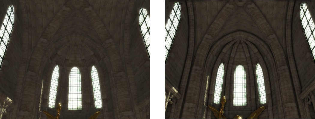
1. You should now be able to compile and run your program to see the effects of using ambient occlusion.

Part 2: Volumetric Lighting

Many real world media do not have solid surface boundaries. These media must be treated as a volume where lighting is a combination of internal lighting events. Most volumetric effects are caused by Participating Media – Particles distributed throughout a region of 3D space.

The distribution of radiance through participating media is defined by 3 effects; Absorption which is the reduction in radiance due to conversion of light to other forms of energy (e.g. heat), Emission which is energy added due to luminous particles and Scattering which causes light heading along one direction to scatter to other directions due to particle collisions.

Scattering is caused by 2 types of events; Out-Scattering which causes light passing through a medium along an incoming direction to be scattered out in other directions. This reduces radiance exiting a differential light beam due to some of it being deflected to other directions. And In-Scattering which increases radiance along a differential beam due to light incoming along other directions being scattered so that it now corresponds to the light beams direction.

Each effect results in different visual phenomena. Trying to handle all such phenomenon is extremely costly but certain effects can be simulated by only taking into account a sub-set of the participating medias light interactions. Light shafts can be simulated purely though in-scattering effects which can simplify the calculations significantly. The total addition to radiance due to in-scattering \(\sigma_{s}\) is given by the source term \(S\left( \overrightarrow{\mathbf{l}} \right)\) based on the phase function \(p\left( \overrightarrow{\mathbf{v}},\overrightarrow{\mathbf{l}} \right)\).

This can be used to calculate the in-scattered light from each light source along a current view direction \(\overrightarrow{\mathbf{v}}\) by splitting the integral into a set of discrete sample positions along the direction vector.

The phase function is used to describe the way light interacts with volumetric participating media. A commonly used phase function is the Henyey-Greenstein phase function. An optimised version of this phase function can be given by the Blasi-Le Saec-Schlick phase function:

1. To implement volumetric light shafts we need to add 2 new programs. The first will be responsible for intersecting the light volume of each spot light and calculating a set of samples within it in order to calculate in-scattering contributions. The second program will then just combine it with the existing accumulation buffer.

GLuint g_uiSpotSSVLProgram;
GLuint g_uiSpotSSVLProgram2;

1. The first step is to create the volumetric light (VL) shader program. This program will work using a full screen quad like the previous AO shader. All it needs is a new Fragment shader that will perform the VL calculations and then write out the values to a texture. This program will calculate light shafts for each of the scenes spot lights so it needs access to the spotlight array and number of spot lights. It also needs access to the spot light shadow map and its associated UBO so that it can determine what parts of the scene are being lit by the light shaft. It also needs the camera position and access to the depth buffer in order to calculate the visible parts of the scene. Finally it also defines 3 constants that are used for later calculations; the first is the step size which is used to define the length of each step through a light volume used to take samples. The second is the input to the phase function \(k\) which is assumed to be constant for the scene and so is hardcoded. This is also assumed for the scattering value \(\sigma_{s}\).

#version 430 core
struct SpotLight {
    vec3 v3LightPosition;
    vec3 v3LightDirection;
    float fCosAngle;
    vec3 v3LightIntensity;
    vec3 v3Falloff;
};
#define MAX_LIGHTS 16
layout(std140, binding = 1) uniform CameraData {
    mat4 m4ViewProjection;
    vec3 v3CameraPosition;
    mat4 m4InvViewProjection;
};
layout(std140, binding = 5) uniform SpotLightData {
    SpotLight SpotLights[MAX_LIGHTS];
};
layout(binding = 6) uniform CameraShadowData {
    mat4 m4ViewProjectionShadow[MAX_LIGHTS];
};
layout(binding = 7) uniform InvResolution {
    vec2 v2InvResolution;
};
 
layout(location = 2) uniform int iNumSpotLights;
 
layout(binding = 6) uniform sampler2DArrayShadow s2aShadowTexture;
layout(binding = 11) uniform sampler2D s2DepthTexture;
 
out vec3 v3VolumeOut;
 
// Volumetric light parameters
const float fStepSize = 0.05f;
float fPhaseK = -0.2f;
float fScatterring = 0.5f; 
#define M_RCP4PI 0.07957747154594766788444188168626f

void main() {
    // Get UV coordinates
    vec2 v2UV = gl_FragCoord.xy * v2InvResolution;
 
    //*** Add VL calculation code here ***
}

1. The body of the new Fragment shader starts of rather simply. It must first use the passed in deferred depth buffer to calculate the visible position. This uses the exact same technique that has been used in previous shaders. It will then loop over each input spot light and then call a new function volumeSpotLight that will be used to determine the volumetric component for each light. Each lights contribution will be combined and then output to a buffer.

// Calculate position from depth
float fDepth = texture(s2DepthTexture, v2UV).r;
fDepth = (fDepth * 2.0f) - 1.0f;
vec2 v2NDCUV = (v2UV * 2.0f) - 1.0f;
vec4 v4Position = m4InvViewProjection * vec4(v2NDCUV, fDepth, 1.0f);
vec3 v3PositionIn = v4Position.xyz / v4Position.w;
 
// Loop over each spot light
vec3 v3RetColour = vec3(0.0f);
for (int i = 0; i < iNumSpotLights; i++) {
    // Calculate volume scattering
    v3RetColour += volumeSpotLight(i, v3PositionIn);
}
 
v3VolumeOut = v3RetColour;

1. This requires making a new function to contain the spot light shaft calculation code. This code will also need access to the light falloff function that we have used in previous tutorials so a copy of that function will need to be created.

vec3 lightFalloff(...)
{
    //*** Copy existing light falloff code here ***
}
 
vec3 volumeSpotLight(in int iLight, in vec3 v3Position)
{
    //*** Add VL calculation here ***
}

1. To determine the contribution of in-scattered light along the current view direction we need to take a series of samples within the light volume and combine them to determine the total effect. To do this efficiently we need to determine how much of the light volume is visible along the current view direction. This is a combination of the size of the light volume and any scene geometry that occludes all or part of each light volume. To start with we need to determine a ray originating from the camera position and travelling along the current pixels view vector. We then clip this ray so that its maximum range is limited from the camera position to the first visible surface.

// Get ray from the camera to first object intersection
vec3 v3RayDirection = v3Position - v3CameraPosition;
float fRayLength = length(v3RayDirection);
v3RayDirection /= fRayLength;
 
// Initialise ray parameters
vec2 v2TRange = vec2(0.0f, fRayLength);

The light volumes created by a spot light can be described by creating a cone with originating point located at the light source and then oriented around the light direction vector. The intersection of a ray and a cone can then be calculated to define the range of a ray that is contained within a light volume. For a cone defined by an originating vertex \(\mathbf{p}_{c}\) a unit length direction \(\overrightarrow{\mathbf{d}_{c}}\) and a cone angle \(\theta\) then the intersection with a ray defined by an originating position \(\mathbf{p}_{0}\) and a direction vector \(\overrightarrow{\mathbf{d}_{r}}\) is given by:

where

This defines a double sided cone where 2 cones spread out from the cone origin position in either the positive or negative cone directions. To limit intersections to only the positive cone an additional inequality is added that constrains the intersection to the positive cone and to only those intersections with the bounded cone region defined by the cones height \(h\).

The quadratic equation can be used to then find the intersections between the ray and the cone. Due to the linear element of the cone intersection equation being defined as a multiple of two the quadratic equation can be simplified such that:

1. Now we have the initial ray parameters we now need to clip the ray against the light volume in order to determine the portion of the current view ray that passes through the light shaft. This is done by treating the spot light volume as a cone and then determining the 2 intersections points with the view ray. We start by precaclulating each of the input values of the quadratic equation. This is done by following the above equations except the only thing we need to take into account is that the input light direction needs to be negated as the input value is directed towards the light whereas the equation needs a vector in the oppsoite direction.

// Calculate quadratic coefficients
vec3 v3LigthDirection = -SpotLights[iLight].v3LightDirection;
vec3 v3FromLightDir = v3CameraPosition - SpotLights[iLight].v3LightPosition;
float fDotLDRD = dot(v3LigthDirection, v3RayDirection);
float fDotLDTLD = dot(v3LigthDirection, v3FromLightDir);
float fDotRDTLD = dot(v3RayDirection, v3FromLightDir);
float fDotTLDTLD = dot(v3FromLightDir, v3FromLightDir);
float fCosSq = SpotLights[iLight].fCosAngle * SpotLights[iLight].fCosAngle;
float fA = (fDotLDRD * fDotLDRD) - fCosSq;
float fB = (fDotLDRD * fDotLDTLD) - (fCosSq * fDotRDTLD);
float fC = (fDotLDTLD * fDotLDTLD) - (fCosSq * fDotTLDTLD);

1. Next we must determine the intersection of the ray with the cone by solving the quadratic equation. The first thing we will do is to check whether there is any intersection with the cone at all by ensuring that that the values in the quadratic equations denominator and within the square root are non-zero and in the case of the square root that they are also greater than zero. This ensures that the results of the quadratic equation will be valid values. If the check passes then we calculate the 2 results of the quadratic equation and then check that they intersect the positive cone and only continue if 1 or both the intersections are valid. If there is only 1 valid intersection then we need to clip out any intersections that occur with the negative cone. This can occur if the view direction is oriented similar to the light direction vector. We need to handle this case by setting the non valid intersection location to a large value. This large value is negated depending on whether the camera is within or outside the light volume. Next we then sort the 2 intersection distances so that they are in the correct near and then far ordering. We then use the spot lights falloff distance to cap the light volume and then clip the ray intersection range to the valid height of the cone. Finally we then clip the 2 cone intersection locations with the actually valid range of the ray to determine the combined intersection of the ray, light volume and scene geometry. The distance between these 2 intersection locations gives the size of the volume the the ray passes through.

// Calculate quadratic intersection points
float fVolumeSize = 0.0f;
float fRoot = (fB * fB) - (fA * fC);
if (fA != 0.0f && fRoot > 0.0f) {
    fRoot = sqrt(fRoot);
    float fInvA = 1.0f / fA;
 
    // Check for any intersections against the positive cone
    vec2 v2ConeInt = (vec2(-fB) + vec2(-fRoot, fRoot)) * fInvA;
    bvec2 b2Comp = greaterThanEqual((fDotLDRD * v2ConeInt) + fDotLDTLD, vec2(0.0f));
    if (any(b2Comp)) {
        // Clip out negative cone intersections
        vec2 v2MinMax = (fDotLDRD >= 0.0)? vec2(2e20) : vec2(-2e20);
        v2ConeInt.x = (b2Comp.x)? v2ConeInt.x : v2MinMax.x;
        v2ConeInt.y = (b2Comp.y)? v2ConeInt.y : v2MinMax.y;
 
        // Sort cone intersections
        float fConeIntBack = v2ConeInt.x;
        v2ConeInt.x = min(v2ConeInt.x, v2ConeInt.y);
        v2ConeInt.y = max(fConeIntBack, v2ConeInt.y);
 
        // Clip to cone height
        vec2 v2ConeRange = (vec2(0.0f, SpotLights[iLight].fFalloffDist) - fDotLDTLD) / fDotLDRD;
        v2ConeRange = (fDotLDRD > 0.0f)? v2ConeRange : v2ConeRange.yx;
        v2ConeInt.x = max(v2ConeInt.x, v2ConeRange.x);
        v2ConeInt.y = min(v2ConeInt.y, v2ConeRange.y);
 
        // Clip to ray length
        v2TRange.x = max(v2TRange.x, v2ConeInt.x);
        v2TRange.y = min(v2TRange.y, v2ConeInt.y);
 
        fVolumeSize = v2TRange.y - v2TRange.x;
    }
}

1. Now we have a value for the size of the light volume that the ray passes through, if this size is greater than zero then the ray intersects the volume and lighting calculations need to be performed.

vec3 v3RetColour = vec3(0.0f);
if (fVolumeSize > 0.0f) {
    //*** Add volume lighting code here ***
}
return v3RetColour;

1. Since we now have the length of the ray that passes through the light volume we need to break this segment into smaller discrete sample locations. We do this by breaking up the ray into a number of small steps which we will then later sample at. To try and reduce the number of samples required we will caclulate the number of steps along the ray to sample at based on the size of the volume that the ray passes through. If it only passes through a small part of the volume then only a few samples should be taken. The larger the size of the volume passed through then the more samples should be taken up to some upper bound. We use the previously defined step size variable to calculate the ideal number of steps. To keep the number of samples low we will use jittered sampling in order to vary the sample locations for each neighbouring pixel. Much like with previous techniques this is used to reduce banding artefacts caused by using a low number of samples. We define a set of 4x4 sample offsets that will vary each pixel within a 4x4 block. We will then later blur the results similar to what we did previously with AO.

//Calculate number of steps through light volume
int iNumSteps = int(max((fVolumeSize / fStepSize), 8.0f));
float fUsedStepSize = fVolumeSize / float(iNumSteps);
 
// Define jittered sampling offsets
const float fSampleOffsets[16] = float[](
    0.442049302f, 0.228878706f, 0.849435568f, 0.192974103f,
    0.001110852f, 0.137045622f, 0.778863043f, 0.989015579f,
    0.463210519f, 0.642646075f, 0.067392051f, 0.330898911f,
    0.533205688f, 0.677708924f, 0.066608429f, 0.486404121f
   );
 
// Get 4x4 sample
ivec2 i2SamplePos = ivec2(gl_FragCoord.xy) % 4;
float fOffset = fSampleOffsets[ (i2SamplePos.y * 4) + i2SamplePos.x ];
fOffset *= fUsedStepSize;

1. Next we calculate the first sample within the light volume. This sample is calculated based on the first intersection location along the ray plus the jittered offset. We then loop over the number of samples, for each sample we calculate the position within the shadow map texture for the corresponding point on the ray. We then check that position against the shadow map to see if it is being lit by the light source. We then combine this value with the amount of light arriving at the sample location and multiplying this by the result of the phase function. This will calculate the amount of light in-scattered along the view direction based on the current point. These values are then later multiplied by the scattering coefficient and the distance between each sample location. The next sample location is then calculated along the ray and the loop continues for all remaining samples with the contribution of each sample being added to the final result.

// Loop through each step and check shadow map
vec3 v3CurrPosition = v3CameraPosition + ((v2TRange.x + fOffset) * v3RayDirection);
for (int i = 0; i < iNumSteps; i++) {
    // Get position in shadow texture
    vec4 v4SVPPosition = m4ViewProjectionShadow[iLight] * vec4(v3CurrPosition, 1.0);
    vec3 v3SVPPosition = v4SVPPosition.xyz / v4SVPPosition.w;
    v3SVPPosition = (v3SVPPosition + 1.0f) * 0.5f;
 
    // Get texture value
    float fText = texture(s2aShadowTexture, vec4(v3SVPPosition.xy, iLight, v3SVPPosition.z));
 
    // Calculate phase function
    float fPhase = M_RCP4PI * (1.0f - (fPhaseK * fPhaseK));
    vec3 v3LightToCurr = normalize(v3CurrPosition - SpotLights[iLight].v3LightPosition);
    float fDotLTCRD = dot(v3LightToCurr, v3RayDirection);
    float fPhaseDenom = 1.0f - (fPhaseK * fDotLTCRD);
    fPhase /= fPhaseDenom * fPhaseDenom;
 
    // Calculate total in-scattering
    vec3 v3LightVolume = lightFalloff(SpotLights[iLight].v3LightIntensity, SpotLights[iLight].v3Falloff, SpotLights[iLight].v3LightPosition, v3CurrPosition);
    v3LightVolume *= fPhase * fText;
 
    // Add to current lighting
    v3RetColour += v3LightVolume;
 
    // Increment position
    v3CurrPosition += fUsedStepSize * v3RayDirection;
}
v3RetColour *= fScatterring * fUsedStepSize;

1. Since we now need the falloff distance of the spot light in order to calculate the light volumes height we need to update the definition of the spot light data within the Fragment shader as well as the deferred Fragment shader and any other shader that uses the spot light data UBO. We will update the existing spot light struct by adding in the new falloff distance value. To efficiently use the available memory space we will pack the new value into existing spare memory so as not to increase the total size of the structure.

struct SpotLight {
    vec3 v3LightPosition;
    vec3 v3LightDirection;
    float fCosAngle;
    vec3 v3LightIntensity;
    vec3 v3Falloff;
    float fFalloffDist;
};

1. Now that the first VL Fragment shader is completed we need to write the second VL Fragment shader. This shader runs as an additional pass using a full screen quad, all it needs to do is read from the input volume light texture and then pass it through to the output. We will use this shader to combine the result of the previous shader and a blur pass into the existing lighting accumulation buffer.

#version 430 core
 
layout(binding = 7) uniform InvResolution {
    vec2 v2InvResolution;
};
layout(binding = 19) uniform sampler2D s2VolumeLightTexture;
 
out vec3 v3VolumeOut;
 
void main() {
    // Get UV coordinates
    vec2 v2UV = gl_FragCoord.xy * v2InvResolution;
 
    // Pass through volume texture
    v3VolumeOut = texture(s2VolumeLightTexture, v2UV).rgb;
}

1. Now we need to modify the host code so that it loads the new shaders. Both new shaders use the same existing Vertex shader that passes through a full screen quad so the only difference between the 2 programs is the corresponding newly created Fragment shaders. You should also ensure that the necessary code to clean-up the programs on exit is added.

1. We now also need to update the definition of the host spot light data to match the one required by the Fragment shader updates. We do this by packing the additional value into the spare 4Bs at the end of the existing falloff vector. Ensure that any usage of SpotLightData is updated accordingly.

struct SpotLightData
{
    aligned_vec3 m_v3Position;
    aligned_vec3 m_v3Direction;
    float m_fAngle;
    aligned_vec3 m_v3Colour;
    aligned_vec3 m_v3Falloff;
    float m_fFalloffDist;
};

1. We also need to update the host code so that a value for the falloff distance is calculated and added to the spot light UBO. This value is already being calculated in the spot light shadow code in order to generate the view-projection matrices for each spot light. We can use this value to update the host spot light falloff distance.

// Update lights falloff value
p_SpotLight->m_fFalloffDist = fFalloff;

1. Within the same section of code once all host spot lights have been updated we just need to then update the UBO buffer with the new falloff data.

// Update spot light UBO with new falloff value
glBindBuffer(GL_UNIFORM_BUFFER, g_SceneData.m_uiSpotLightUBO);
glBufferData(GL_UNIFORM_BUFFER, sizeof(SpotLightData) * g_SceneData.m_uiNumSpotLights, g_SceneData.mp_SpotLights, GL_STATIC_DRAW);

1. Next we need to setup a new framebuffer and output texture that will be used during the VL pass. For this we need a single new framebuffer and a single new texture that will hold the output from the first VL shader program.

// Volumetric lighting data
GLuint g_uiFBOVolLight;
GLuint g_uiVolumeLight;

1. Now we need to add code to the initialise section to setup the new framebuffer and texture. The texture will need to store HDR colour values so we use the same packed floating point format we have used previously. In order to improve the performance of the volumetric light pass we will perform it at half resolution so we allocate the VL texture accordingly. The texture won’t have any mipmaps but we do want to take advantage of BiLinear filtering so we set the texture filtering parameters to GL_LINEAR. Finally we can just bind the VL texture as the framebuffers only output texture. Since there is only one VL texture we can bind it to a texture unit during initialisation just like we did for the AO texture previously. Finally we need to also update the new shaders input uniform so that it knows the correct number of spot lights found in the scene.

// Create volume lighting frame buffer
glGenFramebuffers(1, &g_uiFBOVolLight);
glBindFramebuffer(GL_DRAW_FRAMEBUFFER, g_uiFBOVolLight);
 
// Setup volume lighting texture
glGenTextures(1, &g_uiVolumeLight);
glBindTexture(GL_TEXTURE_2D, g_uiVolumeLight);
glTexStorage2D(GL_TEXTURE_2D, 1, GL_R11F_G11F_B10F, g_iWindowWidth / 2, g_iWindowHeight / 2);
glTexParameteri(GL_TEXTURE_2D, GL_TEXTURE_MIN_FILTER, GL_LINEAR_MIPMAP_NEAREST);
glTexParameteri(GL_TEXTURE_2D, GL_TEXTURE_MAG_FILTER, GL_LINEAR);
glTexParameteri(GL_TEXTURE_2D, GL_TEXTURE_WRAP_S, GL_CLAMP_TO_EDGE);
glTexParameteri(GL_TEXTURE_2D, GL_TEXTURE_WRAP_T, GL_CLAMP_TO_EDGE);
 
// Attach frame buffer attachments
glFramebufferTexture2D(GL_DRAW_FRAMEBUFFER, GL_COLOR_ATTACHMENT0, GL_TEXTURE_2D, g_uiVolumeLight, 0);
 
// Bind volume lighting texture
glActiveTexture(GL_TEXTURE19);
glBindTexture(GL_TEXTURE_2D, g_uiVolumeLight);
glActiveTexture(GL_TEXTURE0);
 
// Set light uniform value
glProgramUniform1i(g_uiSpotSSVLProgram, 2, g_SceneData.m_uiNumSpotLights);

1. You should also add in the required code to clean-up the newly created framebuffer and texture during program exit.

1. In order to use the new VL shader we need to modify the existing deferred rendering pass in the existing GL_RenderDeferred function. The first VL program needs to run after the G-Buffers have been set up but preferably before the accumulation buffers blending operations. We can do this by adding in the first pass after the first AO render pass and right before the second deferred framebuffer is bound. Since we want to improve performance by rendering at half resolution we will first need to update the viewport and then update the resolution UBOs contents accordingly. We can then bind the VL framebuffer and render the full screen quad.

...
// Draw full screen quad
...

// Bind volume light program
glUseProgram(g_uiSpotSSVLProgram);
 
// Half viewport
glViewport(0, 0, g_iWindowWidth / 2, g_iWindowHeight / 2);
vec2 v2InverseRes = 1.0f / vec2((float)(g_iWindowWidth / 2), (float)(g_iWindowHeight / 2));
glBindBuffer(GL_UNIFORM_BUFFER, g_uiInverseResUBO);
glBufferData(GL_UNIFORM_BUFFER, sizeof(vec2), &v2InverseRes, GL_STATIC_DRAW);
 
// Bind frame buffer
glBindFramebuffer(GL_DRAW_FRAMEBUFFER, g_uiFBOVolLight);
glClear(GL_COLOR_BUFFER_BIT);
 
// Draw full screen quad
glDrawElements(GL_TRIANGLES, 6, GL_UNSIGNED_BYTE, 0);

1. Next we need to perform a blur pass on the recently created volumetric light texture. For this we can use the same 2 pass Gaussian blur shader that we created for the Bloom effect in the previous tutorial. To do this we will just bind the blur framebuffer and then bind the volumetric light texture to the texture binding location expected by the blur shader (In this case its location 17). We can then run the 2 blur shader passes exactly in the same way we did in previous tutorials. Once the blur pass has been completed we just need to reset the viewport dimensions and UBO before continuing.

// Bind blur frame buffer and program
glBindFramebuffer(GL_DRAW_FRAMEBUFFER, g_uiFBOBlur);
glUseProgram(g_uiGaussProgram);
 
// Bind volume light texture for blur pass
glActiveTexture(GL_TEXTURE17);
glBindTexture(GL_TEXTURE_2D, g_uiVolumeLight);
 
// Perform horizontal blur
GLuint uiSubRoutines[2] = {0, 1};
glUniformSubroutinesuiv(GL_FRAGMENT_SHADER, 1, &uiSubRoutines[0]);
glClear(GL_COLOR_BUFFER_BIT);
glDrawElements(GL_TRIANGLES, 6, GL_UNSIGNED_BYTE, 0);
 
// Perform vertical blur
glBindFramebuffer(GL_DRAW_FRAMEBUFFER, g_uiFBOVolLight);
glUniformSubroutinesuiv(GL_FRAGMENT_SHADER, 1, &uiSubRoutines[1]);
glBindTexture(GL_TEXTURE_2D, g_uiBlur);
glClear(GL_COLOR_BUFFER_BIT);
glDrawElements(GL_TRIANGLES, 6, GL_UNSIGNED_BYTE, 0);
 
// Reset viewport
glViewport(0, 0, g_iWindowWidth, g_iWindowHeight);
v2InverseRes = 1.0f / vec2((float)g_iWindowWidth, (float)g_iWindowHeight);
glBufferData(GL_UNIFORM_BUFFER, sizeof(vec2), &v2InverseRes, GL_STATIC_DRAW);

// Bind second deferred frame buffer
...

1. Now we just need to add in the final VL pass that will combine the volumetric lighting effects with the existing contents of the accumulation buffer. This can be done directly after the deferred lighting pass adds the direct lighting contribution of each light into the accumulation buffer. Since the blending parameters have already been set up at this point all we need to do is add the code to set the second VL shader program and render the full screen quad.

...
// Draw full screen quad
...
    
// Bind second volume light program
glUseProgram(g_uiSpotSSVLProgram2);
 
// Draw full screen quad
glDrawElements(GL_TRIANGLES, 6, GL_UNSIGNED_BYTE, 0);
 
// Disable blending
...

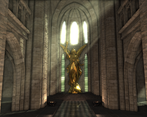
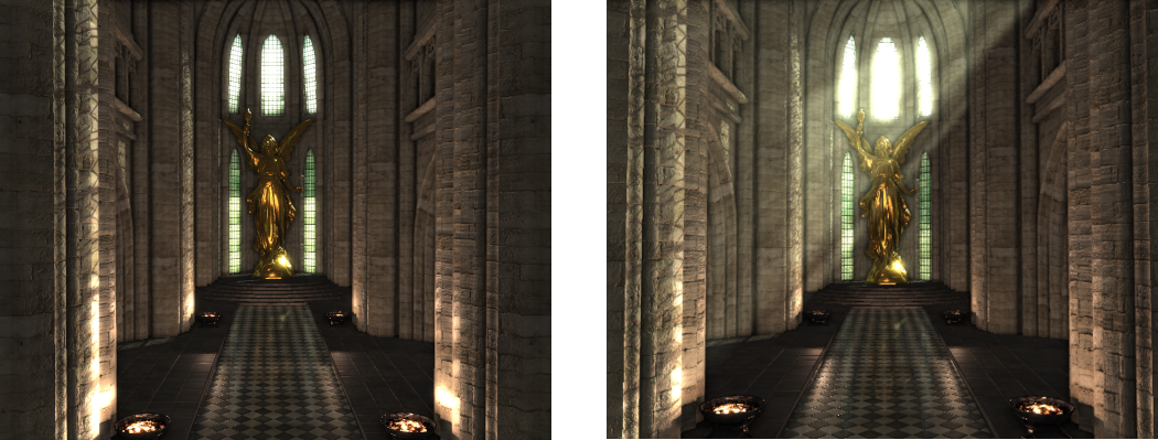
1. You should now be able to compile and run the program in order to see the contribution of the new volumetric light effect.

Extra:

1. Currently ambient occlusion uses a hardcoded constant to scale the size of the hemisphere used to check for local occlusion. Modify this so that it is instead an input uniform which can be user controlled in order to increase or decrease its value. Compare the results of using a different AO radius.

1. The parameter used within the phase function effects the amount of light that is scattered forward or backward from in-scattering events. Positive values cause light to be scattered more forward while negative values cause more light to be scattered backwards. Try changing the value of this parameter and observing its effect. In particular try and observe how it affects lighting when the camera position is located within a light volume and the view is directed either towards or away from the light along its direction vector.

1. The volumetric effect can be improved by combining each samples calculated value with the results of the transparency texture created for each spot light in the extra section of tutorial 7. This will cause the light volume to be correctly coloured based on the colour of the stained-glass windows that each spot light passes through.

Tutorial Solutions